

In a world of interconnected devices, data is being generated at an unprecedented rate. To take advantage of this data, engineers often employ Machine Learning (ML) techniques that allow them to gather valuable insights and actionable information. As the volume of data increases, there is the need to run big data processing pipelines at scale – your laptop just won’t cut it.
To help remedy this, we can use distributed frameworks such as Spark, that allow us to use distributed computing to analyze our data. In this two-part series, you’ll take a small step towards running your data workloads at scale. We present a hands-on tutorial where you’ll learn how to use AWS services to run your processing on the cloud. To do this, we’ll launch an EMR cluster using Lambda functions and run a sample PySpark script. You will need an AWS account to follow this series, as we’ll be using their services.
In this first part, we’ll take a high-level peek at the technologies and architecture, and take a look at a sample problem. In part 2, we’ll dive into the details including architecture and set up of necessary infrastructure.
High-level architecture
Before diving into our sample problem, let’s briefly review the architecture and AWS services involved. We’ll be using Spark, an open-source distributed computing framework for processing large data volumes. Spark can be run on EMR, and we’ll be using its Python API, PySpark. AWS Elastic MapReduce (EMR) is a managed service that simplifies the deployment and management of Hadoop and Spark clusters. Simple Storage Service (S3) is Amazon’s object storage service, which we’ll use to store our PySpark script.
To create the EMR cluster, we’ll use AWS Lambda, a serverless compute service which allows us to run code without the need to provision or manage servers. Using Lambda to create the cluster allows us to define infrastructure as code, so we can define the cluster specifications and configurations once and execute multiple times. We can then launch multiple clusters easily using the same function. Lambda also enables us to define automatic triggers, which we can use to provision clusters automatically based on a set of actions.
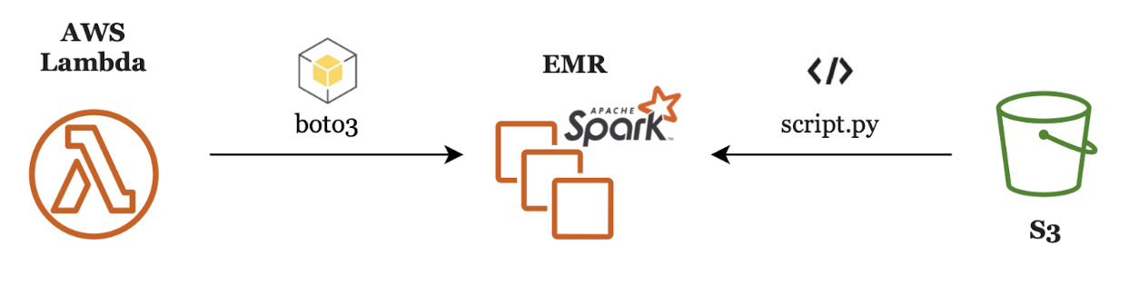
In our sample use case, we’ll create a Python script using AWS’s Python library boto3. This script will be loaded on AWS Lambda and it will trigger the EMR cluster to run our sample PySpark script. The latter will be stored in S3, from where the EMR cluster will retrieve it at runtime.
The problem
We have created a very simple Python script to train a machine learning model using Spark. We’ll generate random data, calculate a linear combination of it, add noise to the results and train a model so that the model can learn how we combined the data. The model should be able to filter out the noise and pretty accurately figure out the coefficients we used to calculate the linear combination of the input data.
Let’s get coding
In this section we’ll walk you through the code, explaining code blocks and commenting on the used functions. At the end you will have the full script available.
1
2
3
4
5
6
7
import argparse
from pyspark.sql import SparkSession
import pyspark.sql.types as T
import pyspark.sql.functions as F
from pyspark.ml.regression import LinearRegression
from pyspark.ml.feature import VectorAssembler
from pyspark.mllib.evaluation import RegressionMetrics
1 import argparse
2 from pyspark.sql import SparkSession
3 import pyspark.sql.types as T
4 import pyspark.sql.functions as F
5 from pyspark.ml.regression import LinearRegression
6 from pyspark.ml.feature import VectorAssembler
7 from pyspark.mllib.evaluation import RegressionMetrics
We’ll be using arguments for our script so we need to import argparse. We’re importing SparkSession to get a hold of the running Spark session. We’ll be using user-defined functions so we need pyspark.sql.types and pyspark.sql.functions. In this example we’ll fit a linear regression model from Spark’s MLlib. The features this model needs are formatted using VectorAssembler. Finally, the model will be evaluated with the built in RegressionMetrics.
 9 NUM_SAMPLES = 1000  # number of samples we'll generate
10
11 if __name__ == "__main__":
12
13  # arguments parsing
14  parser = argparse.ArgumentParser(
15      prog='LinearRegression',
16      description='Randomly generates data and fits a linear regression model using Spark MLlib.'
17  )
18
19    parser.add_argument('--x1', required=True, type=float)
20    parser.add_argument('--x2', required=True, type=float)
21    parser.add_argument('--max_iter', required=True, type=int)
22    args = parser.parse_args()
 9
10
11
12
13
14
15
16
17
18
19
20
21
22
NUM_SAMPLES = 1000  # number of samples we'll generate
if __name__ == "__main__":
    # arguments parsing
    parser = argparse.ArgumentParser(
        prog='LinearRegression',
        description='Randomly generates data and fits a linear regression model using Spark MLlib.'
    )
    parser.add_argument('--x1', required=True, type=float)
    parser.add_argument('--x2', required=True, type=float)
    parser.add_argument('--max_iter', required=True, type=int)
    args = parser.parse_args()
Next, define the number of rows of synthetic data we’ll generate. On lines 14-22 we set up the arguments parser so we can pass parameters to the script. This is a great feature we can use at our advantage when performing tests, and increases the modularity of our code. We’re telling the parser the names of our arguments, if they are required to run the program and their data type. Note the arguments are passed as strings on the Lambda function, and the parser casts them to the specified type.
24  # We're obtaining the spark session.
25  spark = SparkSession
26    .builder
27    .appName("SparkMLExample")
28    .getOrCreate()
24
25
26
27
28
# We're obtaining the spark session.
spark = SparkSession
    .builder
    .appName("SparkMLExample")
    .getOrCreate()
In lines 25-28 we’re obtaining the Spark Session.
30  # create a dataframe
31  num_sample = [[i] for i in range(NUM_SAMPLES)]
32  df = spark.createDataFrame(num_sample)
33 df = df.repartition(4)
30
31
32
33
 # create a dataframe
 num_sample = [[i] for i in range(NUM_SAMPLES)]
 df = spark.createDataFrame(num_sample)
 df = df.repartition(4)
Between lines 31 and 32, we’re initializing a new dataframe with numbers ranging from zero to NUM_SAMPLES – 1. Although this is not directly required, it is an easy way of initializing the dataframe for our purpose. Due to how we’re generating the dataframe, it has a single partition. If that’s the case, all the processing will be done by one machine belonging to the cluster. We’re repartitioning the dataframe into four partitions, this way, the processing will be distributed across the cluster. Note this is correct for our current example, but performing this operation on large amounts of data can result in an expensive shuffle.
34  # generate two columns of random values
35  df = df.withColumn("rand", F.rand())
36  df = df.withColumn("rand2", F.rand())
37  print("displaying generated dataframe...")
38  df.show(10)
34
35
36
37
38
# generate two columns of random values
df = df.withColumn("rand", F.rand())
df = df.withColumn("rand2", F.rand())
print("displaying generated dataframe...")
df.show(10)
On lines 35-36 we’re generating two columns with random values using Spark’s rand function. This generates uniformly distributed random numbers in the range [0,1). We’ll use these as features for our model.
41   # calculate the linear combination of the two generated columns, using the
42  # args x1, x2
43  df = df.withColumn(
44   "raw_result",
45   F.udf(lambda x: args.x1 * x[0] + args.x2 * x[1], T.FloatType())
46  (F.array(F.col('rand'), F.col('rand2'))))
47
48   # generate some random noise to add to the linear combination
49  df = df.withColumn("noise", F.rand())
50
51  # shift the noise from [0,1) to [-0.5,0.5)
52  df = df.withColumn("noise", F.udf(
53   lambda x: x - 0.5, T.FloatType())(F.col('noise')))
54
55  # add the noise to the result
56  df = df.withColumn(
57  "noisy_result",
58   F.udf(lambda x, y: x + y, T.FloatType())(F.col('raw_result'), F.col('noise')))
59
60  print("displaying generated dataframe with labels...")
61  df.show(10)
41
42
43
44
45
46
47
48
49
50
51
52
53
54
55
56
57
58
59
60
61
 # calculate the linear combination of the two generated columns, using the
# args x1, x2
df = df.withColumn(
 "raw_result",
 F.udf(lambda x: args.x1 * x[0] + args.x2 * x[1], T.FloatType())
 (F.array(F.col('rand'), F.col('rand2'))))

 # generate some random noise to add to the linear combination
 df = df.withColumn("noise", F.rand())

# shift the noise from [0,1) to [-0.5,0.5)
 df = df.withColumn("noise", F.udf(
 lambda x: x - 0.5, T.FloatType())(F.col('noise')))

# add the noise to the result
df = df.withColumn(
"noisy_result",
 F.udf(lambda x, y: x + y, T.FloatType())(F.col('raw_result'), F.col('noise')))
print("displaying generated dataframe with labels...")
df.show(10)
On lines 43-46 we’re calculating a linear combination of the two generated columns, using the multipliers passed by arguments. We’re then generating another column with random samples called noise on line 49. As the noise is generated in the range [0,1), we’re subtracting 0.5 to shift the range to [-0.5,0.5). This noise is then added to the linear combination we created on lines 56-58. The purpose of it is to add noise to the data, because if the data was perfect, only a couple of samples would be needed to calculate the coefficients.
63  # create the LinearRegression model to be fit
64  lr = LinearRegression(featuresCol="features", labelCol="label",
65                        solver="l-bfgs", maxIter=args.max_iter)
63
64
65
# create the LinearRegression model to be fit
lr = LinearRegression(featuresCol="features", labelCol="label",
                      solver="l-bfgs", maxIter=args.max_iter)
On line 64, we instantiate a LinearRegression model from Spark’s MLlib to be fit. As the model is fitted with an input dataframe, we’re telling it which columns to search for when given a dataframe, in our case features (inputs) and label (target output).
67  # we need to format the data for the LinearRegression Model
68   vector_assembler = VectorAssembler().setInputCols(
69   ['rand', 'rand2']).setOutputCol('features')
70  df = vector_assembler.transform(df).select(
71    "features", F.col("noisy_result").alias("label"))
67
68
69
70
71
# we need to format the data for the LinearRegression Model
vector_assembler = VectorAssembler().setInputCols(
  ['rand', 'rand2']).setOutputCol('features')
df = vector_assembler.transform(df).select(
     "features", F.col("noisy_result").alias("label"))
MLlib’s models require the data input to be formatted in a specific way, and the VectorAssembler helps us achieve just that. We’re going from two separate columns containing float values to one DenseVector which contains both float features. In line 68 we’re instantiating the VectorAssembler and in line 70 we’re actually using it to transform our data.
73
74
# split the data into training and test set
vdf_train, df_test = df.randomSplit([0.8, 0.2])
73  # split the data into training and test set
74  vdf_train, df_test = df.randomSplit([0.8, 0.2))
As standard practice on ML problems, we’re splitting the data into training and testing. The training data is used to fit the model. The test data is used to evaluate the model on unseen data once it is fitted. It’s kind of simulating what would happen in production. We’re using Spark’s randomSplit to do this, and we’re telling it we want 80% of the data for training and 20% for testing.
76
77
78
79
80
81
82
83
84
85
# fit the model
lr_model = lr.fit(df_train)

# print some info & metrics of the fitting process
print("printing training summary info...")
trainingSummary = lr_model.summary
print(f"number of iterations: {trainingSummary.totalIterations}")
print(f"RMSE: {trainingSummary.rootMeanSquaredError}")
print(f"r2: {trainingSummary.r2}")
print("model coefficients: ", lr_model.coefficients)
76 # fit the model
77 lr_model = lr.fit(df_train)
78
79 # print some info & metrics of the fitting process
80 print("printing training summary info...")
81 trainingSummary = lr_model.summary
82 print(f"number of iterations: {trainingSummary.totalIterations}")
83 print(f"RMSE: {trainingSummary.rootMeanSquaredError}")
84 print(f"r2: {trainingSummary.r2}")
85 print("model coefficients: ", lr_model.coefficients)
This is where the magic happens! In line 77 we’re fitting the model. In the following lines, some info and metrics of the training process are printed to stdout. Note we’re also printing the coefficients learned by the model. If things go well, these should be extremely close to those coefficients which were passed by arguments. They should be close and not exactly equal due to the noise we have introduced to the data.
87
88
89
90
91
92
93
94
95
96
97
98
99
# transform the test data
df_eval = lr_model.transform(df_test)
print("displaying predictions on evaluation data...")
df_eval.show(10)
# format the data so we can evaluate the performance of the model using
# RegressionMetrics
df_eval = df_eval.select('label', 'prediction')
metrics = RegressionMetrics(df_eval.rdd)
print("displaying metrics on test")
print(f"test data RMSE: {metrics.rootMeanSquaredError}")
print(f"test data r2: {metrics.r2}")
87 # transform the test data
88 df_eval = lr_model.transform(df_test)
89 print("displaying predictions on evaluation data...")
90 df_eval.show(10)
91 # format the data so we can evaluate the performance of the model using 92
93 # RegressionMetrics
94 df_eval = df_eval.select('label', 'prediction')
95
96  metrics = RegressionMetrics(df_eval.rdd)
97 print("displaying metrics on test")
98 print(f"test data RMSE: {metrics.rootMeanSquaredError}")
99 print(f"test data r2: {metrics.r2}")
Remember the test data? This is where we use it to evaluate the performance of the model on unknown data. We’re transforming the test dataframe with the already fitted model, which will generate a new column called prediction with the output. Using Spark’s built in RegressionMetrics, we get two metrics for the results on the test data. These are the same metrics as those we got from the training summary, so you can compare the performance of the model on training vs. test data.
 displaying generated dataframe...
+---+-------------------+--------------------+
| _1|               rand|               rand2|
+---+-------------------+--------------------+
|303| 0.4694038640011158|  0.6481209161559824|
| 95| 0.6726286905382153|  0.8981606963845883|
|161| 0.8679103354458326| 0.18119671605635224|
|448|0.30126976391012883|  0.7447454830462397|
|170|  0.864527171418423| 0.07967898764743175|
|131| 0.8658936796366256| 0.19843634271437316|
| 90| 0.9212755414082087|  0.1328917388102402|
|321| 0.4444531531651619| 0.45985908905674244|
| 26| 0.8636854530294522| 0.26834470199928806|
|447| 0.9480941000568025|0.036768371545385814|
+---+-------------------+--------------------+
only showing top 10 rows
displaying generated dataframe with labels...
+---+-------------------+--------------------+----------+-----------+------------+
| _1|               rand|               rand2|raw_result|      noise|noisy_result|
+---+-------------------+--------------------+----------+-----------+------------+
|303| 0.4694038640011158|  0.6481209161559824| 11.175248| 0.06108435|   11.236333|
| 95| 0.6726286905382153|  0.8981606963845883| 15.707894|-0.12919985|   15.578694|
|161| 0.8679103354458326| 0.18119671605635224| 10.491071|  0.3945236|   10.885594|
|448|0.30126976391012883|  0.7447454830462397| 10.460153| -0.0810913|   10.379062|
|170|  0.864527171418423| 0.07967898764743175|  9.442061| 0.43645015|    9.878511|
|131| 0.8658936796366256| 0.19843634271437316|   10.6433|-0.07997194|   10.563328|
| 90| 0.9212755414082087|  0.1328917388102402| 10.541673|0.030807901|    10.57248|
|321| 0.4444531531651619| 0.45985908905674244|  9.043122|-0.29848525|   8.7446375|
| 26| 0.8636854530294522| 0.26834470199928806| 11.320302|-0.43192774|   10.888374|
|447| 0.9480941000568025|0.036768371545385814|  9.848625| 0.11807168|    9.966697|
+---+-------------------+--------------------+----------+-----------+------------+
only showing top 10 rows
printing training summary info...
number of iterations: 4
RMSE: 0.28385880311787814
r2: 0.9954688447304679
model coefficients:  [10.000646699625818,10.005967687529866]
displaying predictions on evaluation data...
+--------------------+---------+------------------+
|            features|    label|        prediction|
+--------------------+---------+------------------+
|[0.00834606519633...|6.4147186|6.2857339058323545|
|[0.06440724048404...| 8.307216| 8.800616841502176|
|[0.11552795484457...| 7.149164| 6.903089763368193|
|[0.12749768801334...|2.6500432|2.8610826921022343|
|[0.16084911790794...| 2.955299| 2.606324673004222|
|[0.18106191852777...| 8.683829| 8.508712313017005|
|[0.19052191329248...|10.528968| 10.22865986628032|
|[0.19501743199211...|11.151053| 11.18943875216736|
|[0.20326177358481...| 9.618211| 9.652048794087703|
|[0.21711604751733...|10.206596|10.217273926029563|
+--------------------+---------+------------------+
only showing top 10 rows
displaying metrics on test
test data RMSE: 0.2923418543882163
test data r2: 0.9945363063793037
Let’s take a glance at the script’s output. The first dataframe being displayed is the result of line 38, and contains the randomly generated inputs. The second one is the result of line’s 61 execution, where we’re displaying the randomly generated values, the linear combination of those, randomly generated noise and the addition of the linear combination and the noise. Training information is then printed, including the number of iterations of the linear regression algorithm, metrics such as RMSE and r2, and the calculated model coefficients. These should be very close to the ones we’re using as inputs x1 and x2. Finally, a portion of the test dataframe is shown, including the inputs (features), the label and the model’s prediction. Metrics on the test data should closely resemble the ones for training.
Conclusion
In this first part of the series, we reviewed the high level architecture we’ll be using to run distributed data processing on AWS. For illustration purposes, we set up an extremely simple example script using pySpark, the Spark API for Python. We reviewed the script and what it does.
In part 2, we’ll dive into the details of running this script on EMR. We’ll explain the technologies to be used and set up the necessary infrastructure to run the example.
By: Maximiliano Palay and Tiziana Romani
Stay ahead of the curve on the latest trends and insights in big data, machine learning and artificial intelligence. Don’t miss out and subscribe to our newsletter!